An illustrative example

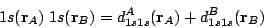
In a LCAO calculation of H₂ carried out with a minimal basis set, the density results:

$$\rho(\mathbf{r}) = \rho_{AA} \; 1s(\mathbf{r}_A) \; 1s(\math... ...thbf{r}_B) + \rho_{BB} \; 1s(\mathbf{r}_B) \; 1s(\mathbf{r}_B)$$ (1)

where $\rho_{IJ}$ are the elements of the density matrix, $\mathbf{r}_I = \mathbf{r}- \mathbf{R}_I$,$\mathbf{R}_I$ stands for the position of the nuclei $I$ ($A$ or $B$), and $1s(\mathbf{r}_I)$is either a $1s$ STO or the corresponding combination of Gaussian primitives.

The first and third terms in (1) contain the spherical charge distributions, $1s(\mathbf{r}_I) \; 1s(\mathbf{r}_I)$ centered at the nuclei $\mathbf{R}_I$. The second term has the two-center charge distribution, $1s(\mathbf{r}_A) \; 1s(\mathbf{r}_B)$ extending along the internuclear axis.

Depicting the values of these distributions along the internuclear axis one has:

The one-center contributions to the density are:

$${\rho'}^I(\mathbf{r}) = \rho_{II} \; 1s(\mathbf{r}_I) \; 1s(\mathbf{r}_I) \hspace*{1cm} I = A, B$$ (2)

The two-center contributions are obtained after partitioning the two-center distribution into two minimally deformed fagments:

$$1s(\mathbf{r}_A) \; 1s(\mathbf{r}_B) = d_{1s1s}^A(\mathbf{r}_A) + d_{1s1s}^B(\mathbf{r}_B)$$ (3)

This partitioning is illustrated in the next figure, where the full distribution, $1s(\mathbf{r}_A) \; 1s(\mathbf{r}_B)$ and the $d_{1s1s}^A(\mathbf{r}_A)$ and $d_{1s1s}^B(\mathbf{r}_B)$ fragments have been plotted along the internuclear axis:

The two-center contributions are:

$${\rho''}^I(\mathbf{r}) = 2 \; \rho_{IJ} \; d_{1s1s}^I(\mathbf{r}_I) + \hspace*{1cm} I,J = A, B; \; I \ne J$$ (4)

The $\rho_{IJ}$ elements of the density matrix can be obtained with different methods. Taking $\xi = 1.2$ and $R = \vert \mathbf{R}_A - \mathbf{R}_B \vert = 1.4$au, and employing the VB, RHF and CI methods for $\rho_{IJ}$ one obtains the following pictures of $\rho^A(\mathbf{r}_A)$, $\rho^B(\mathbf{r}_B)$, and $\rho(\mathbf{r})$ along the internuclear axis:

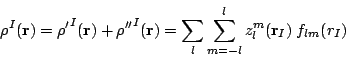
The last step in the method is the expansion of $\rho^I(\mathbf{r}_I)$ in spherical harmonics centered at $\mathbf{R}_I$ times radial factors:

$${\rho'}^I(\mathbf{r}) = \sum_l \sum_{m=-l}^l z_l^m(\mathbf{r}_I) \; f_{lm}(r_I)$$ (5)

This expansion is illustrated in the following figures by drawing the values of the first terms along the internuclear axis. The terms with $l > 0$ have been multiplied by 10 for clarity.