B. Second-order Splitting

The theoretical analysis of the hyperfine splitting considered in this tutorial is valid only for those cases where that electronic Zeeman splitting $(g\beta H)$ is much larger than the hyperfine splitting $(a' m_I)$ (see Eq. (4)). This condition is fulfilled for most of the radicals and the terms $-a M_k$ and $-\sum a_j M_{k,j}$ of Eqs. (6) and (7), which define the position of the lines in relation to the centre of the spectrum $(H_0)$, are denominated first order terms.

For a few radicals, with large coupling constants or when a small magnetic field is used, additional splitting of some lines of the spectrum can occur, giving the called second order effects. In the theoretical treatment of these effects, the Eqs. (6) and (7) are not valid and additional second order terms must be included. These additional terms are proportional to the quotient $-a^2/2H_0$. The resulting equations that replace to the Eqs. (6) and (7), respectively, are:

$$H_k = H_0 - a M_k - \frac{a^2}{2 H_0} \left [ I_k (I_k + 1) - M_k^2 \right ]$$ (11)

and

$$H_k = H_0 - \sum_{j=1}^{r} \left \{ a_j M_{k,j} - \frac{a^... ...} \left [ I_{k,j} (I_{k,j} + 1) - M_{k,j}^2 \right ] \right \}$$ (12)

where $I_k$ or $I_{k,j}$ are the quantum numbers corresponding the module of the nuclear spin angular momentum for the equivalent group of nuclei $j$ in the state $k$ and $M_k = \sum_{i=1}^{n} m_{k,i}$ or $M_{k,j} = \sum_{i=1}^{n} m_{k,j,i}$ are the quantum numbers corresponding to the projection of the nuclear spin angular momentum for the equivalent group of nuclei $j$ in the state $k$.

The second-order splitting can be solved when $-a^2/2H_0$ is similar or larger than the DHpp value of the spectrum lines. For instance, with a magnetic field of 340 mT and a value of DHpp of 0.01 mT, the hyperfine coupling must be larger than 2.6 mT.

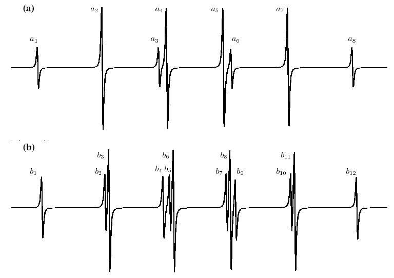
An example of second-order spectrum is that of the neutral radical $\cdot CF_3$ that has three equivalent fluor nuclei and one high hyperfine splitting (14.45 mT). The spectrum of this radical does not give four lines as in the case of the radical $\cdot CH_3$, but when a high resolution spectrum is carried out it consists of six lines due to the second-order splitting².

When the sample is enriched in $^{13}C$, we can detetect also the coupling between the electron spin and the $^{13}C$ nuclear spin which has also a large splitiing (27.16 mT). The spectrum of the radical $\cdot ^{13}CF_3$ simulated like first and second-order is showed in Fig 42. The two possible spin states of $^{13}C$ are: $I = 1/2; \ M = +1/2$ and $I = 1/2; \ M = -1/2$. Spin states of the three equivalent fluor nuclei are more complicated and they are given in Table 5.

Table 5: Nuclear spin states for three equivalent fluor nuclei.

State	$m_{k,i}$			$M_k^a$	$I_k^b$
k	$F_1$	$F_2$	$F_3$
1	$\frac{1}{2}$	$\frac{1}{2}$	$\frac{1}{2}$	$\ \frac{3}{2}$	$\ \frac{3}{2}$
2	$\frac{1}{2}$	$\frac{1}{2}$	$-\frac{1}{2}$	$\frac{1}{2}$	$\ \frac{3}{2}$
3	$\frac{1}{2}$	$-\frac{1}{2}$	$\frac{1}{2}$	$\frac{1}{2}$	$\frac{1}{2}$
4	$-\frac{1}{2}$	$\frac{1}{2}$	$\frac{1}{2}$	$\frac{1}{2}$	$\frac{1}{2}$
5	$-\frac{1}{2}$	$-\frac{1}{2}$	$\frac{1}{2}$	$-\frac{1}{2}$	$\ \frac{3}{2}$
6	$-\frac{1}{2}$	$\frac{1}{2}$	$-\frac{1}{2}$	$-\frac{1}{2}$	$\frac{1}{2}$
7	$\frac{1}{2}$	$-\frac{1}{2}$	$-\frac{1}{2}$	$-\frac{1}{2}$	$\frac{1}{2}$
8	$-\frac{1}{2}$	$-\frac{1}{2}$	$-\frac{1}{2}$	$-\frac{3}{2}$	$\ \frac{3}{2}$

$^a$ $M_k =$ $\sum m_{k,i}$.
$^b$ For some states the assignment of quantum number $I_k$ is arbitrary; for example, the second state $I_2 = 3/2$ and third one with $I_3 = 1/2$ could be interchanged.

Applying the Eq. (12) to the molecule $\cdot ^{13}CF_3$ we can obtain the second-order EPR spectrum. In Table 6 the different signals from first and second-order for the simulated spectrum are given.

Table 6: Displacement with respect to $H_0$ of the 12 signals of the spectrum of the radical $\cdot ^{13}CF_3$

C		F		First order			Second order			Relative
$I_{k}$	$M_{k,j}^b$	$I_{k}$	$M_{k,j}^b$	$H_r -H_0$, Ec. (7)	Signal$^a$ (mT)		Additional Térm. , Eq. (12)	Signal$^a$ (mT)		intensity
$\frac{1}{2}$	$\frac{1}{2}$	$\ \frac{3}{2}$	$\ \frac{3}{2}$	$-\frac{1}{2} a_C - \frac{3}{2} a_F$	$a_1$	-35.25	$- \frac{1}{2} \frac{a_C^2}{2H_0}- \frac{3}{2}\frac{a_F^2}{2H_0}$	$b_1$	-36.26	1
$\frac{1}{2}$	$\frac{1}{2}$	$\ \frac{3}{2}$	$\frac{1}{2}$	$-\frac{1}{2} a_C - \frac{1}{2} a_F$	$a_2$	-20.80	$- \frac{1}{2} \frac{a_C^2}{2H_0}- \frac{7}{2}\frac{a_F^2}{2H_0}$	$b_2$	-22.42	1
$\frac{1}{2}$	$\frac{1}{2}$	$\ \frac{3}{2}$	$-\frac{1}{2}$	$-\frac{1}{2} a_C + \frac{1}{2} a_F$	$a_4$	-6.36	$- \frac{1}{2} \frac{a_C^2}{2H_0}- \frac{7}{2}\frac{a_F^2}{2H_0}$	$b_5$	-7.97	1
$\frac{1}{2}$	$\frac{1}{2}$	$\ \frac{3}{2}$	$-\frac{3}{2}$	$-\frac{1}{2} a_C + \frac{3}{2} a_F$	$a_6$	8.09	$- \frac{1}{2} \frac{a_C^2}{2H_0}- \frac{3}{2}\frac{a_F^2}{2H_0}$	$b_9$	7.09	1
$\frac{1}{2}$	$\frac{1}{2}$	$\frac{1}{2}$	$\frac{1}{2}$	$-\frac{1}{2} a_C - \frac{1}{2} a_F$	$a_2$	-20.80	$- \frac{1}{2} \frac{a_C^2}{2H_0}- \frac{1}{2}\frac{a_F^2}{2H_0}$	$b_3$	-21.50	2
$\frac{1}{2}$	$\frac{1}{2}$	$\frac{1}{2}$	$-\frac{1}{2}$	$-\frac{1}{2} a_C + \frac{1}{2} a_F$	$a_4$	-6.36	$- \frac{1}{2} \frac{a_C^2}{2H_0}- \frac{1}{2}\frac{a_F^2}{2H_0}$	$b_6$	-7.05	2
$\frac{1}{2}$	$-\frac{1}{2}$	$\ \frac{3}{2}$	$\ \frac{3}{2}$	$+\frac{1}{2} a_C - \frac{3}{2} a_F$	$a_3$	-8.09	$- \frac{1}{2} \frac{a_C^2}{2H_0}- \frac{3}{2}\frac{a_F^2}{2H_0}$	$b_{4}$	-9.10	1
$\frac{1}{2}$	$-\frac{1}{2}$	$\ \frac{3}{2}$	$\frac{1}{2}$	$+\frac{1}{2} a_C - \frac{1}{2} a_F$	$a_5$	+6.36	$- \frac{1}{2} \frac{a_C^2}{2H_0}- \frac{7}{2}\frac{a_F^2}{2H_0}$	b$_{7}$	4.74	1
$\frac{1}{2}$	$-\frac{1}{2}$	$\ \frac{3}{2}$	$-\frac{1}{2}$	$+\frac{1}{2} a_C + \frac{1}{2} a_F$	$a_7$	+20.80	$- \frac{1}{2} \frac{a_C^2}{2H_0}- \frac{7}{2}\frac{a_F^2}{2H_0}$	$b_{10}$	19.19	1
$\frac{1}{2}$	$-\frac{1}{2}$	$\ \frac{3}{2}$	$-\frac{3}{2}$	$+\frac{1}{2} a_C + \frac{3}{2} a_F$	$a_8$	+35.25	$- \frac{1}{2} \frac{a_C^2}{2H_0}- \frac{3}{2}\frac{a_F^2}{2H_0}$	$b_{12}$	34.25	1
$\frac{1}{2}$	$-\frac{1}{2}$	$\frac{1}{2}$	$\frac{1}{2}$	$+\frac{1}{2} a_C - \frac{1}{2} a_F$	$a_5$	+6.36	$- \frac{1}{2} \frac{a_C^2}{2H_0}- \frac{1}{2}\frac{a_F^2}{2H_0}$	b$_8$	5.66	2
$\frac{1}{2}$	$-\frac{1}{2}$	$\frac{1}{2}$	$-\frac{1}{2}$	$+\frac{1}{2} a_C + \frac{1}{2} a_F$	$a_7$	+20.80	$- \frac{1}{2} \frac{a_C^2}{2H_0}- \frac{1}{2}\frac{a_F^2}{2H_0}$	$b_{11}$	20.11	2

$^a$Hyperfine splittings $a_C = 27.16$ mT and $a_F = 14.45$ mT in an external magnetic field $H_0 = 340$ mT.
$^b$ $M_{k,j} = \sum m_{k,j,i}$.

In Table 7 we compare the total number of lines and its relative intensities for nuclei with $I=1/2$ considering that the spectrum is first or second order.

Table 7: Intensities for the lines of the spectrum of a molecule with n equivalent nuclei with $I=1/2$.

	First order		Second order
n	Relative intensity	N$^a$	Relative intensity	N$^a$	S$^b$
1	1 : 1	2	1 : 1	2	2
2	1 : 2 : 1	3	1: 1, 1: 1	4	4
3	1 : 3 : 3 : 1	4	1 : 1, 2: 1, 2: 1	6	8
4	1 : 4 : 6 : 4 : 1	5	1: 1,3 : 1,3,2 : 1,3 : 1	9	16

$^a$Number of lines.
$^b$ Sum of the intensities of all lines, $S=2^n$.

Comparing first and second order spectra we can observe the following points:

1. All the lines except the most external are splitting.
2. All the lines except the central one (showed dark character in Table 7) shifted slightly to a smaller magnetic field.
3. The sum of total intensities of all lines of each multiplete $(S)$ is, logically, the same for first order and for second order spectra.
4. The total length of the spectrum remains constant in a first or second-order simulation. In Table 6 we can verify that the length of the spectrum of the radical $\cdot ^{13}CF_3$ is in both cases 70.5 mT.

The simulation of the radical $\cdot ^{13}CF_3$ is presented in Fig 42 according to a first and second-order splitting. This last simulation is most similar to the experimental spectrum.

Figure 42: Simulation of the radical $\cdot ^{13}CF_3$ according to a first order (a) and to second order (b).

It is important to remember that the spectra and the simulations presented in this tutorial correspond exclusively to first order splitting.